Replicating Human-level control through deep reinforcement learning Part 1: Understanding the Loss Function
This series of posts will be to write about my experience replicating an influential reinforcement learning paper published in 2015: Human-level control through deep reinforcement learning. I self-studied CSC421 Deep Learning which had a publically available syllabus and whose lectures were based on accessible research papers, and after completing all the homework, I wanted to do a “capstone.”
The paper was influential because it showed that neural networks were capable of playing games such as pong and breakout at a professional level by only “looking” at the screen (i.e. using the pixels as input).
In part 1, my goal is to provide some intuition behind the loss function’s form (simplified):
\[L = (r + \gamma \max_{a'} Q(s', a', \theta_{fixed}) - Q(s, a, \theta))^2 \;\;\;\; (1)\]In doing so, I will attempt to explain what the Q-value function is, and what deep-Q learning is.
I assume background knowledge on machine learning and neural networks, and being familiar with the basics of reinforcement learning would be helpful, but I do give a brief overview.
What is Reinforcement Learning?
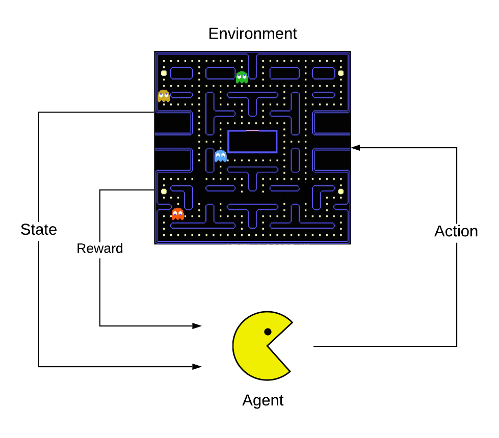
In reinforcement learning, an agent interacts with an environment by observing its state and taking some action. The result of the agent’s action is that it may obtain some reward from the environment and the state of the environment changes. The agent continuously observes the new state and making actions with the goal of maximizing its total reward. This problem formulation can be used to model a myriad of situations. For instance, it can be used to model the classic Atari game pacman. The agent, pacman, has 5 actions: stay still, go up, go down, go left, and go right. The environment is the board, and it is very complex; it has obstacles, ghosts which chase pacman, pellets which cause ghosts to flee and allow pacman to eat them, and points scattered all over the board that pacman must collect.
The strategy or decision-making process that the agent uses to select it’s action is called a policy. Reinforcement learning is teaching a software agent the optimal policy that maximizes its reward.
Reinforcement Learning Theory
There are many online resources for reinforcement learning. You can find many blogs covering the basics in an intuitive way, written in an almost narrative format. Then, there are free textbooks that cover the fundamentals and advanced topics. This section is my best attempt at the former, but sprinkled with rigor insofar as it’s useful to understand the paper.
Problem Formulation
At every time step \(t = 0, 1, 2, ...\) the environment is in some state \(s_t\):
- the agent takes an action \(a_t\)
- the environment moves to some new state \(s_{t+1}\) governed by the dynamics of the environment which is modeled by a probability distribution \(s_{t+1} \sim P(s_{t+1} \vert s_t, a_t)\)
- the agent receives reward \(r_t\) governed by the dynamics of the environment and modeled by a probability distribution \(r_t \sim R(s_t, a_t)\)
The goal of the agent is to maximize the total reward it receives: \(r_0 + r_1 + r_2 + ...\) In reality though, we modify the goal to maximize the total discounted reward: \(r_0 + \gamma r_1 + \gamma^2 r_2 + ...\) where \(\gamma\) is the discount rate satisfying \(0 < \gamma < 1\). In the paper, \(\gamma\) is set to 0.99. I’ve seen it set to other values such as 0.9.
Note: The use of the discount rate can be motivated in a lot of ways. Mathematically, it ensures the sum is not infinite, and that it will converge. Economically, rewards (money) in the future are (is) worth less than rewards (money) right now. Another interpretation is that it models the agent’s uncertainty about the future rewards, and thus, they are worth less. Here is a tangible example to motivate the use of a discount: consider a game where the agent simply needs to move around the board to pickup coins. If the rewards were not discounted, a valid solution for the agent would be to just stay still, because it doesn’t matter when it moves to collect the coins.
The policy of an agent is denoted \(\pi\). The policy can be deterministic \(a_t = \pi(s_t)\) or probabilistic \(a_t \sim \pi(s_t)\).
For the purposes of this blog post, let us assume we somehow obtained a dataset of experiences \(D = [e_1, e_2, e_3, ...]\) where \(e_t = [s_t, a_t, s_{t+1}, r_t]\). How can we train an agent to take actions to optimize the amount of reward it collects?
Example: Pacman
I added this section after feedback from some friends unfamiliar with RL who wanted to see how pacman could be cast using the formulation presented above. Aribitrarily, assume the game is played on a screen that is 200 pixels wide and 200 pixels long.
The state \(s_t\) at each timestep would be \(\mathbb{R}^{200\times200}\). The initial state \(s_0\) would be the initial starting screen which has information about the location of pacman, the ghosts, the points, and the pellets, and the initial reward \(r_0\) would be zero. The agent now needs to decide what to do inside the action space \(\mathbb{A} = \{no-op, move-up, move-down, move-left, move-right\}\). Suppose the agent somehow decided \(a_0 = move-up\), pacman will attempt to execute that action. The environment could deny the action (e.g. because there is an obstacle) and pacman would not change location. Or the action is successful and he moves up. In either case, the environment updates and \(s_1\) is “emitted” or “observed” as well as a reward \(r_1\). For example, if the action was “successful,” \(s_1\) would be similar to \(s_0\) but with pacman and the ghost’s locations slightly perturbed as they moved through the map. If pacman collected a point, then \(r_1\) would be \(>0\). This entire cycle, \([s_0, a_0, s_1, r_1]\) would be called an “experience” consisting of the observed state, the action taken, the resulting state, and the reward collected.
The Q-Value Function
The Q-value function \(Q^\pi(s,a)\) represents the expected discounted reward if an agent currently in state \(s\) takes action \(a\) and then follows policy \(\pi\) for every subsequent action.
\[Q^\pi (s,a) = \mathop{\mathbb{E}} \left[ r_0 + \gamma r_1 + \gamma^2 r_2 + ... \big\vert s_0 = s, a_0 = a \right] \\ = \mathop{\mathbb{E}} \left[ \sum_{t=0}^{\infty} \gamma^t r_t \big\vert s_0 = s, a_0 = a \right]\]In this treatment, I will assume that the policy, state transition and rewards are all deterministic. This will allow us to simplify the equation by not having to marginalize over all possible subsequent actions or resulting states, and to get to a more interpretable equation that elucidates and motivates the form of the loss function presented in the paper. Therefore, we can drop the expectation, and also, let us separate the first term from the sum:
\[Q^\pi (s,a) = r_0 (s,a) + \sum_{t=1}^{\infty} \gamma^t r_t \\ Q^\pi (s,a) = r_0 (s,a) + \gamma \sum_{t=0}^{\infty} \gamma^{t} r_{t+1}\]Let the resulting state be \(s'\), and let \(a' = \pi(s')\). It is easy to see the second term in the equation above is just the discounted Q-value of the resulting state-action pair. That is:
\[Q^\pi (s,a) = r (s,a) + \gamma Q^\pi(s', a') \;\;\;\; (2)\]This is the recursive form of the Q-value function. The goal is to find a policy \(\pi^*\) which maximizes the value of the Q-value function. The optimal Q-value function is:
\[Q^*(s,a) = \sup_\pi Q^\pi(s,a)\]And given \(Q^*\), it is intuitively easy to see that the optimal policy \(\pi^*\) is that which selects the action which maximizes \(Q^*\) i.e. \(\pi^*(s) = \max_a Q^*(s, a)\). Let me reiterate this to emphasize it’s importance: if I have the optimal Q-value function, I also have the optimal policy \(\pi^*\).
Therefore, using equation \((2)\), the optimal Q-value function \(Q^*\) satisfies the following equation:
\[Q^* (s,a) = r (s,a) + \gamma \max_{a'} Q^*(s', a') \;\;\;\; (3)\]Deep-Q Learning And The Loss Function
Deep-Q learning is using a neural network to model the Q-value function i.e. \(Q(s, a, \theta)\). That is it. In the original paper, the neural network actually only accepts the state (input pixels) as input, and it outputs the Q-value of each possible action. Now let’s look at the loss function again.
\[L = (r + \gamma \max_{a'} Q^*(s', a', \theta_{fixed}) - Q(s, a, \theta))^2 \;\;\;\;\]where \(\theta_{fixed} = \theta\) but we do not backpropagate through \(\theta_{fixed}\).
Actually, \(\theta_{fixed}\) is only periodically updated to the “current” weights of the network, for stability purposes.
Does this look familiar? It looks like a squared-error loss, but what is the “label”, and what is the “prediction”? Look at equation (3). The label is \(r + \gamma\max_{a'}Q(s', a', \theta_{fixed})\), i.e. the right-hand side of eqn (3), and the prediction is \(Q(s, a, \theta)\), i.e. the left-hand side of eqn (3).
Then, through repeated backpropagation on a large buffer of experiences, the neural network adjusts it’s weights to solve for Q to make equation (3) true, and the Q function converges to the optimal Q-value function!
Bellman Optimality
The intuition that the neural network will converge comes from the fact that the recursive definition above can be reinterpreted as a Bellman operator operating on the Q function, and the Bellman operator has a property called “contraction” which guarantees convergence to the optimal value in the context of something called value iteration. In value iteration, the Q function is iteratively updated according to the following rule: \(Q_{k+1}(s,a) \leftarrow r(s,a) + \gamma \max_{a'}Q_{k}(s',a')\). I mention it for completeness, but to build your own intuition, I recommend reading about value iteration and using it to solve the problem of an agent escaping from a maze.